Tensorflow v1 vs v2 inference
In tensorflow 1.0, you had to define your model as a graph, and run it using the following syntax:
with tf.Session(...) as sess:
  sess.run(...)
This piece of code basically compiles a graph and puts it on the device that it should be executed on (CPU/GPU).
While compiling the graph, TensorFlow applies various optimizations, like running parallel branches in separate threads, etc. So, as a result, you could expect a better performance of the resulting model. Moreover, such a graph could be saved and run on different platforms without depending on Python at all.
But starting from TensorFlow 2.0, the new eager mode has been introduced (just like in PyTorch). This implies an execution environment that evaluates operations immediately, just like the python interpreter behaves with the python code. And such execution mode could be used, first of all, for development purposes, since we can debug our code easier. For example, the following piece of code should print out “4”, by evaluating the tf.matmul operation immediately:
x = [[2.]]
m = tf.matmul(x, x)
print(f"Result: {x}")
The main disadvantage of such an approach, compared to the “graph” mode - performance.
Here is the inference time comparison for the mobilenetv2 classifier on Intel MacBook 2019 (CPU):
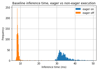
As you can see, the relative difference could be huge - up to ~3-4 times. Also, inference time distribution for the eager mode is spread.
So, you can still develop your model in eager (default) mode in tf 2.0, but you need to enable graph execution when using the training pipeline for inference. Here are some tips on how to switch between eager and graph modes in tf >=2.0:
- call
tf.compat.v1.disable_eager_execution()ortf.compat.v1.enable_eager_execution()before the graph loading / initialization (useful when you load models not trained by you):
class Predictor:
    def __init__(self, path: str) -> None:
        tf.compat.v1.disable_eager_execution()
        self.model = load_model(path)
        ...
- or use the “new” tf.function to wrap up your model after it’s definition, which will trace-compile it to a Tensorflow graph:
from tensorflow.keras import Input, Model
from tensorflow.keras.layers import Flatten, Dense

inputs = Input(shape=(28, 28))
x = Flatten()(inputs)
x = Dense(256, "relu")(x)
x = Dense(256, "relu")(x)
x = Dense(256, "relu")(x)
outputs = Dense(10, "softmax")(x)

model = Model(inputs=inputs, outputs=outputs)

input_data = tf.random.uniform([100, 28, 28])
graph_model = tf.function(model)
print(f"Results: {graph_model(input_data)}")